|
TRACE User Guide
TRACE Version 9.6.1
|
|
TRACE User Guide
TRACE Version 9.6.1
|
Due to general simplifying assumptions during the creation of turbulence models, the prediction accuracy of RANS computations is reduced in the presence of adverse pressure gradient, flow separation and bursting vortices. Consequently, these assumptions lead to a significant degree of epistemic (= structural) uncertainty of the turbulence model. The methodology to quantify these structural uncertainties based on eigenspace perturbations of the Reynolds stress tensor [21] was implemented in TRACE. This approach is a purely physically motivated, data-free forwards method, which tries to estimate the uncertainty bounds by conducting distinct simulations, belonging to the extremal states of the Reynolds stress tensor.
The symmetric Reynolds stress tensor can be decomposed into its anisotropic and isotropic part:
\begin{equation} \uu ij = k \left(a_{ij} + \frac{2}{3} \delta_{ij}\right) \end{equation}
An eigenspace decomposition of the anisotropy tensor \( a_{ij}\) results in
\begin{equation} \uu ij = k \left(v_{in} \Lambda_{nl} v_{li} + \frac{2}{3} \delta_{ij}\right) , \end{equation}
where \( v_{ij}\) represents the eigenvector matrix (composed of the eigenvectors \( v_i\)) and \( \Lambda \) the is the diagonal matrix of eigenvalues \( \lambda_i \). The spectral theorem states that the anisotropy tensor can be constructed as a linear combination
\begin{eqnarray} \Lambda_{ij} &=& v_{ik} a_{kl} v_{lj} \\ &=& \lambda_1 v_1 v_1^T + \lambda_2 v_2 v_2^T + \lambda_3 v_3 v_3^T \\ &=& C_{1_C} \Lambda_{1_C} + C_{2_C} \Lambda_{2_C} + C_{3_C} \Lambda_{3_C} \end{eqnarray}
of its limiting states one-component (1C), isotropic two-component (2C) and isotropic (3C) turbulence with the weights
\begin{eqnarray*} C_{1C} &=& \frac 1 2 (\lambda_1 - \lambda_2) \\ C_{2C} &=& \lambda_2 - \lambda_3 \\ C_{3C} &=& \frac 3 2 \lambda_3 + 1 \end{eqnarray*}
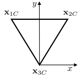
given by the ordered eigenvalues of the anisotropy tensor \( \lambda_1 \leq \lambda_2 \leq \lambda_3 \) [2]. A barycentric map can be used as a tool to visualize the anisotropy tensor. The three vertices of the triangle are the basis matrices \( \Lambda_{1_C} \), \( \Lambda_{2_C} \) and \( \Lambda_{3_C} \) and can be identified as three points \(\mathbf{x_{1C}} = (x_{1C}, y_{1C})\), \(\mathbf{x_{2C}} = (x_{2C}, y_{2C})\) and \(\mathbf{x_{3C}} =(x_{3C}, y_{3C})\). Applying a convex combination of the limiting turbulent states, each physical realizable state of turbulence can be determined in barycentric coordinates by
\begin{eqnarray} \mathbf{x} &=& \mathbf{x_{1C}} C_{1_C} + \mathbf{x_{2C}} C_{2_C} + \mathbf{x_{3C}} C_{3_C} \\ &=& \mathbf{x_{1C}} \frac 1 2 (\lambda_1 - \lambda_2) + \mathbf{x_{2C}} (\lambda_2 - \lambda_3) + \mathbf{x_{3C}} (\frac 3 2 \lambda_3 + 1) \\ &=& \mathbf{B} \lambda_i \end{eqnarray}
Choosing the vertices to be \(\mathbf{x_{1C}} = (- \frac 1 2, \frac{\sqrt{3}}{2})\), \(\mathbf{x_{2C}} = (\frac 1 2, \frac{\sqrt{3}}{2})\) and \(\mathbf{x_{3C}} =(0, 0)\) results in a barycentric map, which is oriented as follows:
This means for the transformation matrix:
\begin{equation} \mathbf{B} = \left( \begin{array}{rrr} \frac 1 4 & \frac 3 4 & -\frac 1 2 \\ \frac{\sqrt{3}}{4} & \frac{\sqrt{3}}{4} & -\frac{\sqrt{3}}{2} \end{array}\right) \end{equation}
The perturbation approach seeks to shift the turbulent state inside the barycentric triangle with a relative distance \( \Delta_B \) between the current state \( \mathbf{x} \) and the turbulent cornes (= target state) \( \mathbf{x}_{t} \in (\mathbf{x_{1C}}, \mathbf{x_{2C}}, \mathbf{x_{3C}}) \).
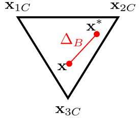
The perturbed state can be determined by
\begin{equation} \mathbf{x^*} = \mathbf{x} + \Delta_B (\mathbf{x_{t} - \mathbf{x}}) \quad \text{with} \quad \Delta_B \in [0,1] \end{equation}
The perturbed eigenvalues can then be recomposed by
\begin{equation} \lambda^*_i = \mathbf{B}^{-1} \mathbf{x^*} \end{equation}
with
\begin{equation} \mathbf{B}^{-1} = \frac 1 9 \left(\begin{array}{rr} -9 & 5 \sqrt{3} \\ 9 & -\sqrt{3}\\ 0 & -4 \sqrt{3} \end{array}\right) \end{equation}
Since the turbulent production term for the turbulent kinetic energy is defined as
\begin{equation} P_k = - \uu ij \frac{\partial u_i}{\partial x_j} = - \uu ij \cdot \mathbf{S}_{ij} \quad \text{,} \end{equation}
with the strain rate tensor \(\mathbf{S}_{ij} = \frac 1 2 (\frac{\partial u_i}{\partial x_j} + \frac{\partial u_j}{\partial x_i})\), the turbulent production is dependent on the alignment of the eigenvectors of the Reynolds stress tensor and the strain rate tensor. Because linear eddy viscosity turbulence models rely on the Boussinesq assumptions, the eigenvectors of the Reynolds stress tensor are identical to the ones of the strain rate tensor. On the one hand the production gets maximized, if the eigenvectors of the Reynolds stress tensor (which are coincide with the eigenvectors of the anisotropy tensor) correspond with the strain rate tensor. On the other hand \( P_k \) can be minimized by permuting \( v_1 \) and \( v_3 \). Therefore, the perturbation framework for the eigenvectors distinguishes between a maximized (unperturbed, compared to the baseline model) production \( P_{k_{max}} \) and minimized (perturbed) turbulent production \( P_{k_{min}} \).
The perturbed eigenvalues and eigenvectors are used afterwards to compose the perturbed anisotropy tensor
\begin{equation} a_{jl}^* = v^*_{in} \Lambda^*_{nl} v^*_{li} \end{equation}
The perturbed Reynolds stress tensor can then be reconstructed:
\begin{equation} \uu ij^* = k \left(a_{jl}^* + \frac{2}{3} \delta_{ij} \right) \end{equation}
When the eigenspace perturbation approach is used, TRACE replaces the computation of the baseline turbulent production by using the perturbed Reynolds stresses
\begin{equation} P^*_k = - \uu ij^* \cdot \mathbf{S}_{ij} \end{equation}
Additionally, the turbulent fluxes are computed using the perturbed Reynolds stress tensor as well (comparable to Reynolds stress models).
 1.9.1
1.9.1