|
TRACE User Guide
TRACE Version 9.6.1
|
|
TRACE User Guide
TRACE Version 9.6.1
|
Approaches of varying degrees of abstraction can be employed to include the effects of film-cooling in numerical simulations. Conceptually, the simplest approach is to include and resolve the cooling ducts or slots directly in the computational domain. The difficulty with this approach is the effort that must be expended to mesh the individual holes and include them in the computational domain. At their inflow a conventional inflow boundary condition is employed.
This strategy allows for the most detailed description of the geometry and flow physics and may therefore be expected to provide the highest degree of accuracy. Ultimately, however, this accuracy depends on the quality and resolution of the mesh and discretization schemes used in a given simulation. The major disadvantage of this approach is that the inclusion of the individual cooling holes both vastly increases the complexity of the computational domain and greatly increases the total number of computational cells. Alternatively a bleed boundary condition and a volume-based source model are included to model such flows. A comparative study can be found in Becker et al. [4] .
The film cooling model allows for the simulation of an arbitrary number of discrete film cooling holes. Any grid can be used, since the effects are modeled by the introduction of source terms in the vicinity of the cooling hole. However, the grid resolution has to be sufficient to resolve the relevant flow phenomena. Depending on the goal of the simulation a few cells per cooling hole may be sufficient, especially if the wall temperatures around the film cooling hole are not of particular interest. The following paragraphs describe how the model works and how to adapt it to different cooling hole geometries. More information on how to control and use the film cooling model can be found n StartFilmCoolingModel .
In this mode, only cells adjacent to the wall get a source term. This is done by marking all cells that fit into a 2D pattern describing the geometry of the film cooling hole exit. This pattern is constructed by a Fourier series with up to 4 coefficients, which allows users to approximate a wide range of different hole geometries. There will be some errors in the approximation of the geometry, but those will usually be below the practicable grid resolution for most use cases of the model.
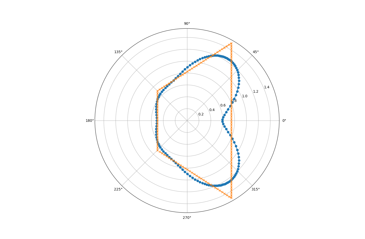
In contrast to the first option, the source terms for mass, momentum and energy are distributed in an arbitrary volume. In the simplest case, this volume is defined by the cooling hole geometry and does not change depending on the flow conditions. Alternatively, a more flexible, but also more complex, system can be used. Here, cells are defined by 2D shapes strung along a "centerline" trajectory, up to 1.5 times the diameter of the cooling hole:
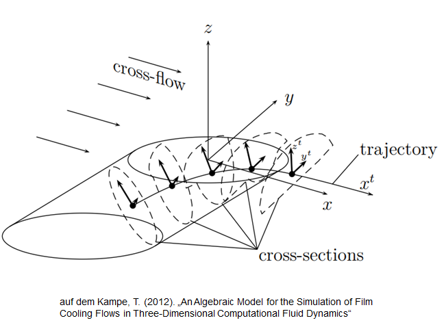
Both the trajectory and the shape of the film cooling jet is determined by a set of parameters and the solution. Recalculating which cells actually get a source term is the most expensive part of the model. Therefore, the user can specify in which intervals this will be done. Additionally, the number of discrete points used to describe the trajectory can be changed.
The parameters defining the trajectory and shape of the area with source terms are given in a separate, editable library. This library is dynamically linked to TRACE, no recompilation or relinking of the TRACE executable is necessary. To use the film cooling model with the standard library found in contrib/filmCoolingParameterLibrary, the makefile in that folder has to be run and the newly created libCooling.so has to be added to the environment variable "LD_LIBRARY_PATH". After this, the film cooling model can be activated by the control file commands given in StartFilmCoolingModel.
A few more steps are necessary to implement a custom set of parameters. This short step-by-step description can be used as a guide:
1: Add new identifier to CoolingHoleType enumerator in filmCoolingLibrary.h
2: Add new function declarations to the end of filmCoolingLibrary.h
3: Add those new functions to the switch-case in getTrajectoryParameters and getModelSourceTermDistributionParameters in filmCoolingLibrary.c. Whenever a film cooling hole with the new enum is simulated, this branch of the switch statement will be executed. Functions for the trajectory, the shape and for turbulence variables are necessary, but they can set parameters to 0 in step 4. This is useful for deactivating a source term, e.g. for the turbulence equations. The original model had more parameters for e.g. a velocity distribution within the film cooling jet. Those parameters are calculated in the library, but not used in TRACE.
4: Copy the filmCoolingParametersCylindrical.c file and give it an apropriate name. This will be used as a blueprint to implement the new set of parameters. At the bottom of the file, replace the function names with those stated in step 3. Also replace the names of the sub-functions called within. All input variables should be left unchanged, unless a special implementation requires it.
5: Implement the sub-functions renamed in step 4. Usually it should be sufficient to change the name and the parameters of the already existing functions. It is also possible to set constant values, so 0 to deactivate any turbulence source term is of course also valid. All available input data can be found in filmCoolingLibrary.h under the struct CoolingHoleDataLibrary. The definition of the functions using those parameters can be found in the dissertation of auf dem Kampe, as given above.
6: Add the new filmCoolingParametersNewShape files to the makefile. In total this is necessary in 3 locations, as marked in the picture below.
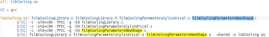
7: Recompile by running the make file and follow the procedure given in Film cooling parameter library
To model individual cooling holes, or alternatively a localized group of cooling holes, a simple boundary condition based on the Newton-Raphson method and extrapolation from the inner solution is employed. The aim of the boundary condition is to ensure that the converged solution on the boundary satisfies the user specified values of mass flow rate, stagnation temperature and flow direction. To impose this goal the stagnation temperature residual \( R^{BC}\) is defined as the difference between the current local value of \( T_{\mathrm{tot},\:\mathrm{abs}} = T_{\mathrm{tot},\:\mathrm{abs}}(T,\dot{m}^*, A^*_{H}, \Omega)\), computed from the transformed relative values, and the prescribed value \( T_{\mathrm{tot},\:\mathrm{abs}}^{*}\), e.g.
\begin{equation} R^{BC} = T_{\mathrm{tot},\:\mathrm{abs}}(T,\dot{m}^*, A^*_{H}, \Omega) - T_{\mathrm{tot},\:\mathrm{abs}}^{*} , \end{equation}
where \(\dot{m}^*\) is the prescribed massflow rate and \(A^*_{H}\) is the area of the cooling hole. Introducing the Newton-Raphson method the static temperature \(T_B\) is obtained iteratively as
\begin{equation} T^{n+1}_B = T^{n}_B - \frac{R^{BC}(T^n_B,\dot{m}^*, A^*_{H}, \Omega)}{\partial R^{BC}/\partial T_B} \end{equation}
in which the Jacobian, \(\partial R^{BC}/\partial T_B\), is computed numerically using finite differences. Following the extrapolation of the static pressure from the first inner cell to the boundary, the value of density, \(\rho_B\), is computed using the computed values of pressure and temperature together with the appropriate gas law. Finally, the velocity components are computed as
\begin{equation} \mathbf{u}_B = \frac{\dot{m}^*}{\rho_B A^*_{H}}\frac{\mathbf{r}_B}{{\mathbf{r}_B}\cdot{\mathbf{n}}} , \end{equation}
where \({\mathbf{r}_B}\) is the unit direction vector of the bleed and \({\mathbf{n}}\) is the local surface normal.
Using this approach to represent the individual cooling holes the complexity of the computational domain can be greatly reduced and far fewer computational cells are required than if the cooling cooling holes are directly meshed. However, as the boundary condition prescribes only a single averaged state at each individual cooling hole (or selectively even a group of cooling holes) the approach can not be expected to entirely accurately capture the local flow details at the boundaries of the computational domain.
In TRACE the cooling source terms have been implemented as volumetric source terms. Using a block container idea the associated control volume can be easily assembled. It comprises either a single block, multiple blocks or all the blocks of one specific blade row. As input parameters the mass flow rate \(\dot{m}_{VSM}\) and an averaged temperature \( T_{VSM}\) as well as a velocity vector \(\mathbf{v}\) stated in the relative frame of reference have to be given. The velocity vector can either be a constant vector ( \({\mathbf v}_i = {\mathbf v}\)) or the local flow velocities can be used instead.
The quantities are distributed volume weighted to all cells of the control volume ( \( CV\)). Therefore the source terms of continuity, momentum and energy equations are defined for a single cell as follows
\begin{eqnarray}\label{VolumeSourceTerms} \dot{m}_i & = & \frac{V_i}{V_{CV}} \dot{m}_{VSM}\\ S_{{VSM,\dot{m}}_i}&=& \frac{\dot{m}_i}{V_i} = \frac{\dot{m}_{VSM}}{V_{CV}} = S_{VSM,\dot{m}}\\ {\mathbf S}_{{VSM,M}_i} &=& \frac{\dot{m}_i}{V_i} {\mathbf v}_i = S_{VSM,\dot{m}} {\mathbf v}_i\\ S_{{VSM,E}_i} &=& \frac{\dot{m}_i}{V_i} (h + \frac{1}{2} \left|{\mathbf v}_i\right|^2 - \frac{1}{2}\left(\omega r_i\right)^2)\\ & = & S_{VSM,\dot{m}} (h + \frac{1}{2} \left|{\mathbf v}_i\right|^2 - \frac{1}{2}\left(\omega r_i\right)^2) \end{eqnarray}
The source term of the energy equation \({S_{VSM,E}}\) in Eqn. VolumeSourceTerms is defined as the rothalpy. The enthalpy \({h}\) is computed from the given temperature \({T_{VSM}}\) depending on the equation of state.
The main advantages of this volumetric approach are its simplicity and flexibilty. It can be used either like the bleed boundary condition to model local film cooling effects or as a global source term requiring neither the explicit resolution of the cooling holes nor the individual modelling with a local boundary condition.
In general however as also only a single averaged state is used to represent each source region the approach cannot be expected to capture the local flow details. For the global effects of the film cooling in a turbine this again greatly reduces the complexity of the computation domain and requires significantly fewer computation cells than if the cooling holes were directly resolved in the computational domain. Furthermore, as only the averaged effect of the cooling holes must be specified, rather than boundary values for each individual cooling hole, the pre-processing effort is greatly reduced in comparison to the boundary condition approach.
 1.9.1
1.9.1